Linear Regression
Data, goal and model
Given a dataset of $N$ observations $\{\mathbf{x}_n, t_n\},\; n = 1,\dots,N$.
The goal to find a function $y: \mathbb{R}^D \rightarrow \mathbb{R}$ such that $t \approx y(\mathbf{x}, \mathbf{w})$.
The linear regression model has the form: \[ \begin{equation} y = \mathbf{w}^T\mathbf{x}, \; \mathbf{x} \in \mathbb{R}^D\tag{0}\label{0} \end{equation} \]
The most popular estimation method is to minimize sum of squared residuals:
\[ \begin{equation} \text{RSS}(\mathbf{w}) = \sum_n^{n = N} (t_n - \mathbf{w}^T \mathbf{x}_n)^2 \rightarrow min \tag{1}\label{1} \end{equation} \]
Maximum likelihood and least squares
We assume that the target variable $t$ is given by a function $y(\mathbf{x}, \mathbf{w})$ with additive Gaussian noise: \[ \begin{equation} t = y(\mathbf{x}, \mathbf{w}) + \epsilon, \; \epsilon \sim \mathcal{N}(0, \sigma^2) \tag{2}\label{2} \end{equation} \] In other words: \[ \begin{equation} p(t|\mathbf{x}, \mathbf{w}, \sigma^2) = \mathcal{N} (t|y(\mathbf{x}, \mathbf{w}),\sigma^2). \tag{3}\label{3} \end{equation} \]
Making the assumption that our data points are drawn independently from the distribution (\ref{3}), we obtain the following expression for the likelihood function \[ p(\mathbf{t}|\mathbf{\mathcal{X}}, \mathbf{w}, \sigma^2) = \prod^{N}_{n = 1}\mathcal{N} (t_n|\mathbf{w}^T \mathbf{x}_n,\sigma^2) \]
Recall Gaussian distribution function: \[ \begin{equation} p(x|\mu, \sigma) = \frac{1}{\sigma \sqrt{2 \pi}}\exp{-\frac{(x - \mu)^2}{2\sigma^2}}. \tag{4}\label{4} \end{equation} \]
Let us substitute it to likelihood expression and take a logarithm:
\[ \begin{equation} ln (p(\mathbf{t}|\mathbf{w}, \sigma^2)) = -\frac{N}{2} ln(2\pi\sigma^2) - \frac{1}{2\sigma^2} \sum_{i = 1}^{N} (t_i - \mathbf{w}^T \mathbf{x}_i)^2. \tag{5}\label{5} \end{equation} \] Here we can see that maximization of the likelihood function is equivalent to minimizing a sum-of-squares error function.
Analytical solution
We can write the residual sum-of-squares as:
\[ \begin{equation} \text{RSS}(\mathbf{w}) = (\mathbf{t} − \mathbf{X}\mathbf{w})^T (\mathbf{t} − \mathbf{X}\mathbf{w}) \tag{6}\label{6} \end{equation} \]
where $\mathbf{X}$ is $n \times D$ design matrix, $\mathbf{t}$ is $n \times 1$ vector.
Setting the first derivative to zero:
\[ \begin{equation} \frac{\partial \text{RSS}(\mathbf{w})}{\partial \mathbf{w}} = −2\mathbf{X}^T (\mathbf{t} − \mathbf{X}\mathbf{w}) \tag{7}\label{7} \end{equation} \]
we get the solution:
\[ \begin{equation} \mathbf{\hat w} = (\mathbf{X}^T \mathbf{X})^{-1} \mathbf{X}^T \mathbf{t} \tag{8}\label{8} \end{equation} \]
Here are the problems:
- what if $\mathbf{X}^T \mathbf{X}$ is singular (number of observations greater than number of features or two or more features are linearly dependent) ?
- what if the dimensions of $\mathbf{X}$ are too large
Bias variance tradeoff
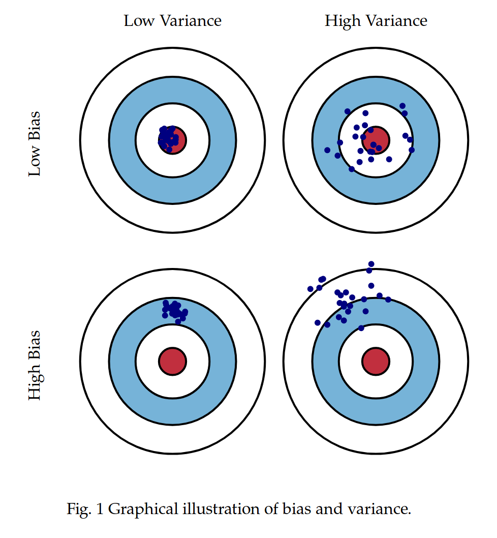
Assuming $\hat{y}$ is the approximation of $y$ we are looking for we can decompose the error $\mathbf{x}$ into bias and variance.
\[
\begin{split}
\text{Err}\left(\textbf{x}\right) &=& \mathbb{E}\left[\left(t - \hat{y} \left(\textbf{x}\right)\right)^2\right] \\
&=& \mathbb{E}\left[t^2\right] + \mathbb{E}\left[\left(\hat{y}\left(\textbf{x}\right)\right)^2\right] - 2\mathbb{E}\left[t\hat{y}\left(\textbf{x}\right)\right] \\
&=& \mathbb{E}\left[t^2\right] + \mathbb{E}\left[\hat{y}^2\right] - 2\mathbb{E}\left[t\hat{y}\right]
\end{split} \tag{9}\label{eq9}
\]
\[
\begin{split}
\mathbb{E}\left[t^2\right] &=& \text{Var}\left(t\right) + \mathbb{E}\left[t\right]^2 = \sigma^2 + y^2 \\
\mathbb{E}\left[\widehat{y}^2\right] &=& \text{Var}\left(\widehat{y}\right) + \mathbb{E}\left[\widehat{y}\right]^2 \\
\end{split} \tag{10}\label{eq10}
\]
\[
\begin{split}
\text{Var}\left(t\right) &=& \mathbb{E}\left[\left(t - \mathbb{E}\left[t\right]\right)^2\right] \\
&=& \mathbb{E}\left[\left(t - y\right)^2\right] \\
&=& \mathbb{E}\left[\left(y + \epsilon - y\right)^2\right] \\
&=& \mathbb{E}\left[\epsilon^2\right] = \sigma^2
\end{split} \tag{11}\label{eq11}
\]
\[ \begin{equation} \mathbb{E}[t] = \mathbb{E}[y + \epsilon] = \mathbb{E}[y] + \mathbb{E}[\epsilon] = y \tag{12}\label{12} \end{equation} \]
\[
\begin{split}
\mathbb{E}\left[t\hat{y}\right] &=& \mathbb{E}\left[\left(y + \epsilon\right)\hat{y}\right] \\
&=& \mathbb{E}\left[f\hat{y}\right] + \mathbb{E}\left[\epsilon\hat{y}\right] \\
&=& y\mathbb{E}\left[\hat{y}\right] + \mathbb{E}\left[\epsilon\right] \mathbb{E}\left[\hat{y}\right] = y\mathbb{E}\left[\hat{y}\right]
\end{split} \tag{13}\label{eq13}
\]
\[
\begin{split}
\text{Err}\left(\textbf{x}\right) &=& \mathbb{E}\left[\left(t - \hat{y}\left(\textbf{x}\right)\right)^2\right] \\
&=& \sigma^2 + y^2 + \text{Var}\left(\hat{y}\right) + \mathbb{E}\left[\hat{y}\right]^2 - 2y\mathbb{E}\left[\hat{y}\right] \\
&=& \left(f - \mathbb{E}\left[\hat{y}\right]\right)^2 + \text{Var}\left(\hat{y}\right) + \sigma^2 \\
&=& \text{Bias}\left(\hat{y}\right)^2 + \text{Var}\left(\hat{y}\right) + \sigma^2
\end{split} \tag{14}\label{eq14}
\]
Regularization
Ridge regression model
\[ \begin{equation} RSS_{ridge}(\mathbf{w}) = \frac{1}{2}\sum_{n = 1}^{N}(t_n − \mathbf{w}^T \mathbf{x}_n)^2 + \frac{\lambda}{2} \mathbf{w}^T\mathbf{w} \end{equation} \]
Analytic solution
\[ \begin{equation} \mathbf{\hat w} = (\mathbf{X}^T \mathbf{X} + \lambda^2 \mathbf{I})^{-1} \mathbf{X}^T \mathbf{t} \end{equation} \]
- sensitive to noise
Lasso regression model
\[ \begin{equation} RSS_{lasso}(\mathbf{w}) = \frac{1}{2}\sum_{n = 1}^{N}(t_n − \mathbf{w}^T \mathbf{x}_n)^2 + \frac{\lambda}{2} ||\mathbf{w}||_{L_1} \end{equation} \]
- insensitive to noise
- leads to sparse model (if $\lambda$ is large some of coefficients become close to $0$)
ElasticNet regularization
\[ \begin{equation} RSS_{elastic}(\mathbf{w}) = \frac{1}{2}\sum_{n = 1}^{N}(t_n − \mathbf{w}^T \mathbf{x}_n)^2 + \frac{\lambda_1}{2} \mathbf{w}^T\mathbf{w} + \frac{\lambda_2}{2} ||\mathbf{w}||_{L_1} \end{equation} \]
Metrics
- MSE
- MAE
- Root MSE
- RMSLE \[ \begin{equation} RMSLE = \sqrt{ \sum_{n = 1}^{N} (\log{(1 + t_n)} - \log{(1 + y_n)})^2} \end{equation} \]
- MSPE \[ \begin{equation} MAPE = \frac{1}{n} \sum_{n = 1}^{N} \left(\frac{t_n - y_n}{t_n}\right)^2 \end{equation} \]
- MAPE \[ \begin{equation} MAPE = \frac{1}{n} \sum_{n = 1}^{N} \left|\frac{t_n - y_n}{t_n}\right| \end{equation} \]
- SMAPE \[ \begin{equation} SMAPE = \frac{1}{n} \sum_{n = 1}^{N} \frac{2 |t_n - y_n|}{|t_n + y_n|} \end{equation} \]
Coefficient of determination ($R^2$)
R-squared is the “percent of variance explained”.
\[ \begin{equation} R^2 = \frac{Var(mean) - Var(fit)}{Var(mean)} \end{equation} \]
Pros & Cons
- [+] easy to interpret
- [+] computational efficient
- [-] gets affected by outliers
- [-] does not work well with correlated features