Singular Value Decomposition (SVD). Principal Component Analysis (PCA).

I. SVD

Singular value decomposition (SVD) is a method of representing a matrix as a series of linear transformations that expose the underlying meaning-structure of the matrix. These transformations are rotation (matrix $U$), rescaling (matrix $\Sigma$) and rotation again (matrix $V^T$).

Let $A_{m \times n}$ be a data matrix with $m$ rows (documents or examples) and $n$ columns (terms or features).

SVD represents an input matrix as a product of three matrices (it is always possible to do for real matrix): \[ \begin{equation} A_{m \times n} = U_{m\times m} \Sigma_{m\times n} V_{n\times n}^T \end{equation} \] where

$U_{m \times m}$ is an orthonormal matrix of left singular vectors (eigenvectors of $AA^T$)
$\Sigma_{m \times n}$ is a diagonal matrix and contains the square-roots of the eigenvalues of $AA^T$ and $A^T A$
$V_{n \times n}^T$ is an orthonormal matrix of right singular vectors (the eigenvectors of $A^T A$)

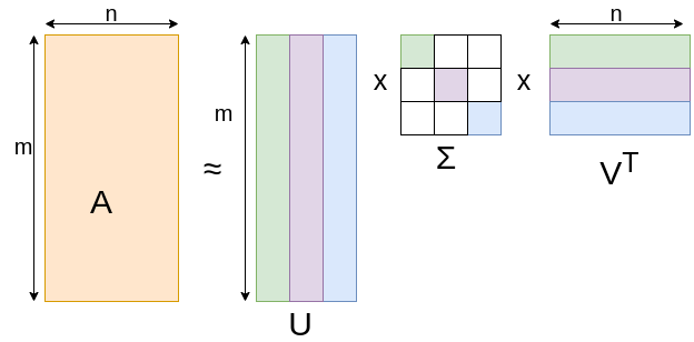
Depending on $m$, $n$, $r = rank(A)$, some of the left singular vectors may “collapse” to zero (see figure). This happens when the matrix $A$ does not have full rank for instance, since then its range must be a subspace of $R^m$ with dimension $r < n$.

svd_1

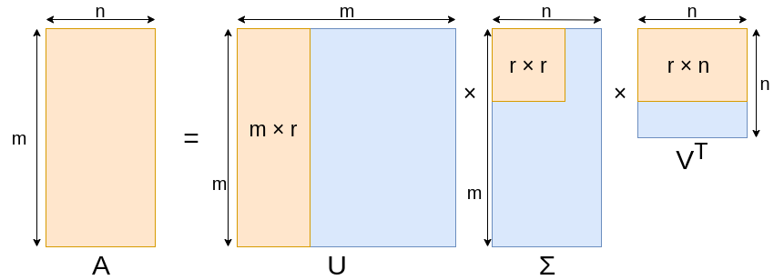
For convenience we assume that $m \geq n$ and here is the “compact” version of SVD: \[ \begin{equation} A_{m \times n} = U_{m \times r} \Sigma_{r \times r} V_{n \times r}^T, \end{equation} \] where

$U_{m \times r}$ is the matrix of left singular vectors, $r$ is the number of latent factors
$\Sigma_{r \times r}$ is diagonal matrix of the singular values. Also $r$ is the rank of matrix $A$
$V_{n \times r}^T$ is the matrix of right singular vectors

All three matrices are unique. $U$ and $V$ are column orthonormal. Entities of $\Sigma$ matrix are positive and sorted in decreasing order.

Geometrical intuition

(Detailed explanation by Gregory Gundersen)

Any linear transformation can be thought of as simply stretching or compressing or flipping a square, provided we are allowed to rotate it first. This is the geometric essence of SVD.

Let $\mathbf{v}_1$ and $\mathbf{v}_2$ be orthogonal vectors in some two-dimensional vector space $S$. We know that any two orthogonal vectors form a basis in two-dimensional space. Linear operator $A$ maps $S$ to $Q$: \[ \begin{split} A \mathbf{v}_1 &= \mathbf{u}_1 \sigma_1\ \;\; A \mathbf{v}_2 &= \mathbf{u}_2 \sigma_2 \end{split} \tag{1}\label{eq1} \] where $\mathbf{u}_1$ and $\mathbf{u}_2$ are the unit vectors in $Q$. And $\sigma_1$ and $\sigma_2$ are the lengths of the new vectors in space $Q$.

Any vector $\mathbf{x}$ can be written as: \[ \begin{equation} \mathbf{x} = (\mathbf{x} \cdot \mathbf{v}_1) \mathbf{v}_1 + (\mathbf{x} \cdot \mathbf{v}_2) \mathbf{v}_2 \tag{2}\label{eq2} \end{equation} \] where $\mathbf{x} \cdot \mathbf{v}$ is just a projection $\mathbf{x}$ on to $\mathbf{v}$.

Multiplying both sides by $A$ rewrite the previous equation: \[ \begin{equation} A \mathbf{x} = (\mathbf{x} \cdot \mathbf{v}_1) A \mathbf{v}_1 + (\mathbf{x} \cdot \mathbf{v}_2) A \mathbf{v}_2 \end{equation} \] \[ \begin{equation} A \mathbf{x} = (\mathbf{x} \cdot \mathbf{v}_1) \mathbf{u}_1 \sigma_1 + (\mathbf{x} \cdot \mathbf{v}_2) \mathbf{u}_2 \sigma_2 \end{equation} \] \[ \begin{equation} A \mathbf{x} = \mathbf{u}_1 \sigma_1 \mathbf{v}_1^{\top} \mathbf{x} + \mathbf{u}_2 \sigma_2 \mathbf{v}_2^{\top} \mathbf{x} \tag{3}\label{eq3} \end{equation} \] In the last equation we use the option $\mathbf{x} \cdot \mathbf{v}_1 = \mathbf{x}^{\top} \mathbf{v}_1 = \mathbf{v}_1^{\top} \mathbf{x}$.

Dividing the equation $\ref{eq3}$ by $\mathbf{x}$, we get \[ \begin{equation} A = \mathbf{u}_1 \sigma_1 \mathbf{v}_1 + \mathbf{u}_2 \sigma_2 \mathbf{v}_2 \tag{4}\label{eq4} \end{equation} \] Equation $\ref{eq4}$ can be transformed to canonical SVD form: \[ A = \begin{bmatrix} \mathbf{u}_1 & \mathbf{u}_2 \end{bmatrix} \begin{bmatrix}\sigma_1 & 0 \\ 0 & \sigma_2 \end{bmatrix} \begin{bmatrix} \mathbf{v}_1^{\top} \\ \mathbf{v}_2^{\top} \end{bmatrix} \tag{5}\label{eq5} \]

Applications

svd_0 Let us take as example traditional customer-product data where $m$ customers consume $n$ products (for example movie rating matrix, grocery store products). One hypothesizes that there are really only $r$ underlying basic factors like age, sex, income, etc. that determine a customer’s behavior. An individual customer’s behavior is determined by some weighted combination of these underlying factors. That is, a customer’s purchase behavior can be characterized by a $r$-dimensional vector where $r$ is much smaller that $m$ and $n$. The components of the vector are weights for each of the basic factors. Associated with each basic factor is a vector of probabilities, each component of which is the probability of purchasing a given product by someone whose behavior depends only on that factor. More abstractly, $A$ is an $m\times n$ matrix that can be expressed as the product of two matrices $U$ and $V$ where $U$ is an $m \times r$ matrix expressing the factor weights for each customer and $V$ is a $r \times n$ matrix expressing the purchase probabilities of products that correspond to that factor. One twist is that $A$ may not be exactly equal to $UV$ , but close to it since there may be noise or random perturbations[4].

II. PCA. Relation Between SVD and PCA.

Let us assume that our data centered and represented by matrix $\mathbf A_{m \times n}$. The covariance matrix is given by $\mathbf C = \frac{\mathbf A^\top \mathbf A}{m-1}$ and it can be diagonalized: \[ \begin{equation} \mathbf C = \mathbf V \mathbf \Lambda \mathbf V^\top, \end{equation} \] where

$\mathbf V$ is a matrix of eigenvectors or principal directions (each column is an eigenvector)
$\mathbf \Lambda$ is a diagonal matrix with eigenvalues $\lambda_i$ in the decreasing order on the diagonal.

Projections of the data on the principal directions are called principal components. The $j$-th principal component is given by $j$-th column of $\mathbf A \mathbf V$. The coordinates of the $i$-th data point in the new PC space are given by the $i$-th row of $\mathbf A \mathbf V$.

Performing SVD we get: \[ \begin{equation} \mathbf A = \mathbf U \mathbf \Sigma \mathbf V^\top, \end{equation} \] \[ \begin{equation} \mathbf C = \frac{\mathbf V \mathbf \Sigma \mathbf U^\top \mathbf U \mathbf \Sigma \mathbf V^\top}{m-1} = \mathbf V \frac{\mathbf \Sigma^2}{m-1}\mathbf V^\top, \end{equation} \]

We can see that PCA diagonalizes the covariance matrix of $\mathbf A$ and looks for the major axes along which our data varies.

Principal components are given by $\mathbf A \mathbf V = \mathbf U \mathbf \Sigma \mathbf V^\top \mathbf V = \mathbf U \mathbf \Sigma$.

Another way to implement PCA:

Data normalization and centering
Covariance matrix computation
Computation of eigenvalues and eigenvectors
Sorting them from largest to smallest and choosing components. Choose $k$ eigenvectors with the largest eigenvalues (dimension reduction).
To compute Principal Components form a feature vector using the eigenvectors we chose to keep. Multiply the original data by the eigenvectors to re-orient data onto the new axes