Recurrent neural networks
The reason why we use RNNs is processing sequential data like texts, voice and music records, video records etc. We can think of RNNs that they have a memory which captures information what has been calculated so far. In other words when RNNs process an element in the sequence the output depends on the calculations performed on the previous elements in the sequence.
\[
\begin{split}
&a^{(t)} = W_{hh} h^{(t-1)} + W_{xh}x^{(t)} + b_h \\\
&h^{(t)} = f(a^{(t)}) \\\\
&o^{(t)} = W_{hz} h^{(t)} + b_z \\\
&z^{(t)} = g(o^{(t)})
\end{split}
\tag{1}\label{eq1}
\]
Where
- $x^{(t)}$ is the input at time step $t$
- $h^{(t)}$ is the hidden state at time step $t$, $f$ is nonlinear function such as $\sigma$ or $tanh$
- $o^{(t)}$ is the intermediate term. Used to calculate $z^{(t)}$
- $z^{(t)}$ is the output(prediction) at the time step $t$ produced with function $g$ (e.g. $softmax$)
Backpropagation
In RNNs loss is calculated for each output $z^t$. To account with multiple losses RNNs Backpropagation through time is used.
Let $L(\cdot)$ be the chosen loss function and the objective function is expressed as \[ \begin{equation} L(x,y) = \sum_{t=1}^{T} L(y^t, z^t)\tag{2}\label{eq2} \end{equation} \] We start with its derivative with respect to $W_{hz}$ and bias $b_z$:
\[ \begin{equation} \frac{\partial L}{\partial W_{hz}} = \sum_{t=1}^{T}\frac{\partial L}{\partial z^t} \frac{\partial z^t}{\partial W_{hz}} \tag{3}\label{eq3} \end{equation} \]
\[ \begin{equation} \frac{\partial L}{\partial b_z} = \sum_{t=1}^{T}\frac{\partial L}{\partial z^t} \frac{\partial z^t}{\partial b_z} \tag{4}\label{eq4} \end{equation} \]
Now let us derive the derivative w.r.t. $W_{hh}$. \[ \begin{equation} \frac{\partial L^{t+1}}{\partial W_{hh}} = \sum_{k=1}^{t}\frac{\partial L^{t+1}}{\partial z^{t+1}} \frac{\partial z^{t+1}}{\partial h^{t+1}} \frac{\partial h^{t+1}}{\partial h^{k}} \frac{\partial h^{k}}{\partial W_{hh}} \end{equation} \]
\[ \begin{equation} \frac{\partial L}{\partial W_{hh}} = \sum_{t=1}^{T}\sum_{k=1}^{t+1}\frac{\partial L^{t+1}}{\partial z^{t+1}} \frac{\partial z^{t+1}}{\partial h^{t+1}} \frac{\partial h^{t+1}}{\partial h^{k}} \frac{\partial h^{k}}{\partial W_{hh}}\tag{5}\label{eq5} \end{equation} \]
Now we turn to derive the gradient w.r.t.$W_{xh}$. (We consider just the time step $t$). Since $h^{t}$ and $x^{t+1}$ both make a contribution to $h^{t+1}$ and we get: \[ \begin{equation} \frac{\partial L^{t+1}}{\partial W_{xh}} = \frac{\partial L^{t+1}}{\partial h^{t+1}} \frac{\partial h^{t+1}}{\partial W_{xh}} + \frac{\partial L^{t+1}}{\partial h^{t+1}} \frac{\partial h^{t+1}}{\partial h^{t}} \frac{\partial h^{t}}{\partial W_{xh}} \end{equation} \]
Finally we get \[ \begin{equation} \frac{\partial L}{\partial W_{xh}} = \sum_{t=1}^{T} \sum_{k=1}^{t+1}\frac{\partial L^{t+1}}{\partial z^{t+1}} \frac{\partial z^{t+1}}{\partial h^{t+1}} \frac{\partial h^{t+1}}{\partial h^{k}} \frac{\partial h^{k}}{\partial W_{xh}} \tag{6}\label{eq6} \end{equation} \]
Such a vanilla form of RNN suffers from vanishing and exploding gradients. It happens because of matrix multiplication over the sequence in ($\ref{eq6}$) (term $\frac{\partial h^{t+1}}{\partial h^{k}}$). And it is the reason why it is difficult to capture long term dependencies.
Long Short-Term Memory (LSTM)
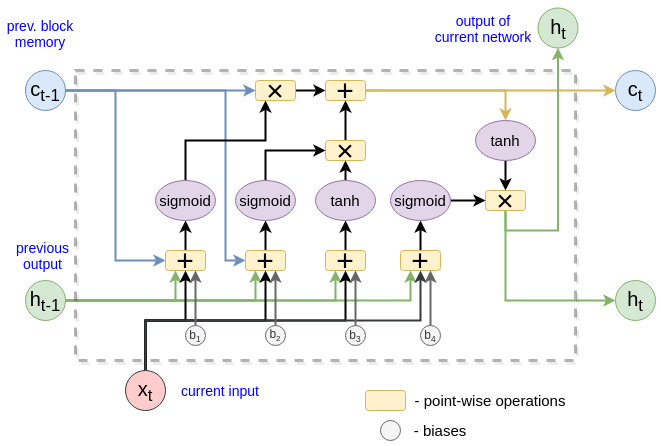
The key idea behind LSTM is that there is a path $C_{t-1} \rightarrow C_{t}$ (at the picture below). It allows the information to flow unchanged if our LSTM multiply the old memory $C_{t-1}$ with the vector that is equal to $1$.
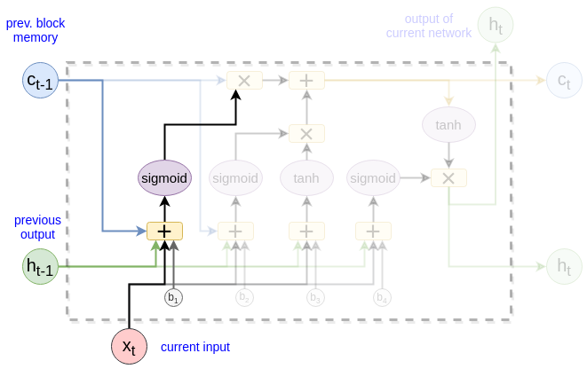
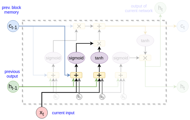
Forget gate
This is the first step. It decides what information to be thrown away from the cell state.
This gate returns the value between $(0, 1)$ and that is why the sigmoid function is used:
\[
\begin{equation}
f_t = \sigma(W_{wf}x_t + W_{hf}h_{t-1} + W_{cf}c_{t-1} + b_f)
\tag{0}\label{eq7}
\end{equation}
\]
Input gate and Candidate cell state
This step controls how much the new memory should influence the old memory. This has two parts. The input gate decides which value from input should be used to modify the memory. Next, a tanh layer creates a vector of new candidate values (or in other words the new memory) $\hat c$
\[
\begin{split}
&i_t = \sigma(W_{xi}x_t + W_{hi}h_{t-1} + b_i)\\\
&\hat c_t = tanh(W_{xc}x_t + W_{hc}h_{t-1} + b_{\hat c})\\\
\end{split}
\tag{1}\label{eq8}
\]
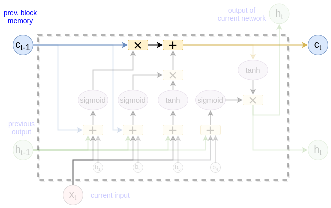
The next state computing
\[
\begin{equation}
c_t = f_t * c_{t-1} + i_t * \hat c_t
\tag{2}\label{eq9}
\end{equation}
\]
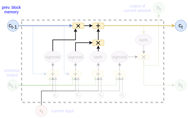
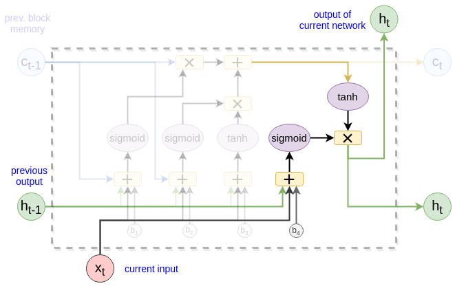
The output
This output $h_t$ is based on our cell state $c_t$
\[
\begin{split}
&o_t = \sigma(W_{xo}x_t + W_{ho}h_{t-1} + b_o)\\\
&h_t = o_t * tanh(c_t)\\\
\end{split}
\tag{3}\label{eq10}
\]