Basics of statistics
1. Combinatorics reminder
Permutations
Permutations are all the possible ways elements in a set can be arranged, where the order is important. The number of permutations of subsets of size $k$ drawn from a set of size $n$ is given by \[ A^k_n = nPk = \frac{n!}{(n-k)!} \]
Combinations
Combinations are all the possible ways to select items from a collection, such that (unlike permutations) the order of selection does not matter. The number of combinations of subsets of size $k$ drawn from a set of size $n$ is given by: \[ C^k_n = nCk = \binom{n}{k} = \frac{n!}{k!(n-k)!} \]
1. Expectation, variance, skewness, kurtosis
Expectation:
if $X$ is discrete random variable:
\[
\begin{equation}
E[X] = \sum_{x}^{\infty} x \, p_X(x)
\end{equation}
\]
if $X$ is continuous random variable:
\[
\begin{equation}
E[X] = \int_{-\infty}^{\infty} x \, f_X(x)\, dx
\end{equation}
\]
Variance: \[ \begin{equation} Var(X)=E[(X-E[X])^2] = E[X^2]-(E[X])^2 \end{equation} \]
Standardized moment is the $n$-th central moment divided by $\sigma^n$:
\[ \begin{equation} \frac{\mu_n}{\sigma^n} = \frac{E[(X - \mu)^n]}{\sigma^n} \end{equation} \]
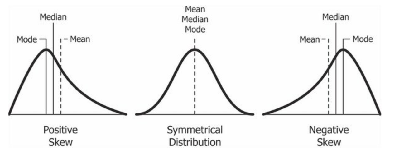
Skewness (Pearson’s moment coefficient of skewness or the third standardized moment):
\[
\begin{equation}
\tilde{\mu}_3 = E\left[\frac{X - \mu}{\sigma}\right]^3 = \frac{E[(X - \mu)^3]}{E[(X - \mu)^2]^{3/2}}
\end{equation}
\]
Kurtosis
\[ \begin{equation} Kurt[X] = E\left[\frac{X - \mu}{\sigma}\right]^4 = \frac{E[(X - \mu)^4]}{E[(X - \mu)^2]^{2}} \end{equation} \]
Kurtosis is a measure of whether the data are heavy-tailed or light-tailed relative to a normal distribution. That is, data sets with high kurtosis tend to have heavy tails, or outliers.
The kurtosis for a standard normal distribution is three: $Kurt[X] - 3 = 0$.
2. Covariance
Is a way to classify three types of linear relationship:
- When $Cov$ is positive relationship has a positive slope
- When $Cov$ is negative relationship has a negative slope
- When $Cov$ is $0$ there is no relationship
Covariance of two jointly distributed real-valued random variables
\[ \begin{equation} Cov(X, Y) = E((X - E(X))(Y-E(Y))) \end{equation} \]
Covariance of two datasamples
\[ \begin{equation} Cov(X, Y) = \frac{\sum_i(X-X_i)(Y-Y_i)}{n - 1} \end{equation} \]
Covariance matrix
Data is represented as matrix $X \in \mathbb{R}^{n \times d}$, $n$ is the number of samples, $d$ is the dimension of feature space (or number of features).
Calculation of covariance matrix is expressed as: \[ \begin{equation} C = \frac{1}{n-1} \sum^{n}_{i=1}{(X_i-\bar{X})(X_i-\bar{X})^T} = \frac{1}{n-1} X^T X \end{equation} \]
Here $C_{i,j} = \sigma(x_i, x_j)$ is the entity of the covariance matrix, $C \in \mathbb{R}^{d \times d}$.
3. Correlation
For population
Given a pair of random variables $X,Y$; \[ \begin{equation} Corr(X, Y) = \frac{Cov(X, Y)}{\sigma_X\sigma_Y} \end{equation} \]
For sample
Given paired data ${(x_1, y_1), \dots , (x_n , y_n)}$ consisting of $n$ pairs; \[ \begin{equation} r_{xy}= \frac{\sum_{i=1}^{n} (x_i - \overline{x})(y_i - \overline{y})} {\sqrt{\sum_{i=1}^{n} (x_i - \overline{x})^2(y_i - \overline{y})^2}} \end{equation} \]
4. Mean Absolute Deviation (MAD)
\[ \begin{equation} MAD(X) = \frac{1}{n}\sum_i^n|x_i - m(X)| \end{equation} \] here $m(X)$ is central point. The choice of measure $m(X)$ depends on our data set.
5. Interquartile range (IQR)
Quartiles divide a rank-ordered data set into $4$ equal parts. The interquartile range (IQR) is the difference between the first quartile and third quartile. $Q_1$ is the median of the $n$ smallest numbers. $Q_3$ is the median of the $n$ largest numbers. \[ \begin{equation} IQR(X) = Q_3 - Q_1 \end{equation} \]
Judging outliers in a dataset
\[ \begin{equation} outliers < Q_1 - 1.5\cdot IQR(X)\;or\; outliers > Q_3 + 1.5\cdot IQR(X) \end{equation} \]
6. Z-score
Z-score (or standard score) represents how many standard deviations a given measurement deviates from the mean
\[ \begin{equation} z = \frac{x_i - \mu}{\sigma} \end{equation} \]
7. Limit theorems
The law of large numbers
As the number of identicaly ditributed, randomly generated numbers increases, their sample mean approaches their theoretical mean.
Theorem.
Let $X_1, X_2, \dots X_i$ be a sequence of independent random variables with $E(X_i) = \mu$ and $Var(X_i) = \sigma^2$. Let $\overline{X_n} = \frac{\sum_i^nX_i}{n}$. Then for any $\epsilon > 0$ \[ \begin{equation} P(|\overline{X_n} - \mu| > \epsilon) \rightarrow 0, \; as \; n \rightarrow \infty \end{equation} \]
The Central Limit Theorem (CLT)
It states that, under certain conditions, the sum of a large number of random variables is approximately normal. Or in terms of population: if you have a population with mean $\mu$ and standard deviation $\sigma$ and take sufficiently large random samples from the population with replacement, then the distribution of the sample means will be approximately normally distributed.