Boosting and Additive Trees. AdaBoost.
The general idea of boosting is to create a strong classifier from a number of weak classifiers. A weak classifier produces prediction that slightly better than random guessing.
To make highly accurate model Adaboost combines many weak classifiers, so that weak classifier takes into account the errors of the previous weak classifier.
The most common weak learner algorithm used with Adaboost is Decision Tree with one level or decision stumps (just a node and two leaves).
The boosting algorithm Adaboost
The idea is to set weights to both classifiers and samples in a way that forces classifiers
to focus on observations that are difficult to correctly classify. In other words weight of
a sample indicates how important it is to be correctly classified.
- Given the training set $(x_0, y_0),\dots, (x_m, y_m)$, where $x_i \in X$, $y_i \in \{-1, 1\}$
- Initialize weights of samples $D_1(i) = 1/m$, for $i=1,\dots, m$. It means the samples are equally important
- For $t=1,\dots, T$:
- Train a weak learner using distribution $D_t$
- Get weak hypothesis $h_t \rightarrow \{-1, 1\}$
-
Aim: select $h_t$ with low weighted error: $\epsilon_t = Pr_{i\sim D_t}(h_t(x_i) \neq y_i)$.
-
Choose weight of hypothesis (classifier): \[ \begin{equation} \alpha_t = \frac{1}{2}\ln (\frac{1-\epsilon_t}{\epsilon_t}) \tag{1}\label{eq1} \end{equation} \] It defines how much say classifier $h_t$ has in final classification.
- Update weights of samples. For $i=1,\dots, m$: \[ \begin{equation} D_{t+1}(i) = \frac{D_{t}(i)\exp(-\alpha_t y_i h_t(x_i))}{Z_t} \tag{2}\label{eq2} \end{equation} \] where $Z_t$ is a normalization factor (chosen so that $D_{t+1}$ will be a distribution).
- Final hypothesis: \[ \begin{equation} H(x) = sign(\sum_{t=1}^T \alpha_t h_t(x)) \tag{3}\label{eq3} \end{equation} \]
The most interesting part is in step 3.1. To create the first stump in the forest
we start with finding the feature that does the best classification of our samples.
For instance, if our dataset contains four features, we determine which one
is the best by creating four stumps. Then we calculate the Gini index for these
four stumps and select the stump with the lowest value of Gini index as the first
stump of the forest.
Now we need to determine the stumps weight in final classification, this is done by calculating
it’s total misclassification error:
\[
\begin{equation}
\epsilon_t = \frac{\sum_{i=1}^m D_t(i)I(y_i \neq h_t(x_i))}{\sum_{i=1}^m D_t(i)}\tag{4}\label{eq4}
\end{equation}
\]
and substituting the result into $(\ref{eq1})$.
Since all weights add up to $1$ the misclassification error $\epsilon_t$ is between $0$ for perfect stump
and $1$ for worst stump. We finish the first iteration by updating the weights of samples. To compute the expression
$(\ref{eq2})$ we first compute the expression in numerator and then sum up the result values to get normalization
coefficient $Z_t$.
In the picture below there is a graph of $\exp(-\alpha_t y_i h_t(x_i))$ depending on the sign of $y_i h_t(x_i)$.
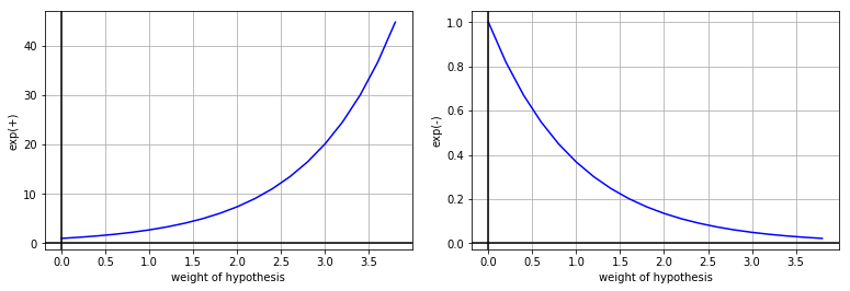 It is easy to see when the value of $y_i h_t(x_i)$ is positive i.e. the signs of both ground truth value $y_i$ and
hypothesis $h_t(x_i)$ match, then we scale the previous sample with small number and vice versa.
It is easy to see when the value of $y_i h_t(x_i)$ is positive i.e. the signs of both ground truth value $y_i$ and
hypothesis $h_t(x_i)$ match, then we scale the previous sample with small number and vice versa.