Decision Trees
There are two types of decision trees:
- Classification tree solves classification problems. Predicted outcome is the category of the object it belongs to. In a classification tree each leaf has discrete category.
- Regression tree solves regression problems. Predicted outcome is real number. In a regression tree each leaf represents a numeric value.
1. Decision tree building. Classification tree.
Decision tree algorithms transform raw data to rule based decision tree. The decision of making data splits heavily affects a tree’s accuracy. There are several algorithms to decide how to split a node in two or more subnodes. Splitting criteria (metric) is different for classification and regression trees.
1.1 Information Gain. Entropy.
Shannon’s entropy is defined as: \[ \begin{equation} S = -\sum_{i}^C p_i log_2(p_i), \end{equation} \] where $C$ is the number of classes, $p_i$ is the probability to pick an element of class $i$. It can be interpreted as measure of uncertainty or randomness in data.
Information gain is the reduction in entropy (or another impurity criteria) of the system : \[ \begin{equation} IG = S_0 - \sum_{g=1}^{g=Groups} \frac{N_g}{N}S_g \end{equation} \]
For example, consider a coin toss: the probability to get a head is 0.5 and it is equal to the probability to get a tail. It means the uncertainty takes its maximum value 1, since there is no chance to precisely determine the outcome.
Another toy example. Circles color in dependence on their coordinates:
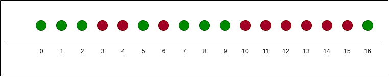 There are 17 circles: 9 red and 8 green.
The entropy of initial state is equal to
There are 17 circles: 9 red and 8 green.
The entropy of initial state is equal to
\[ \begin{equation} S_0 = - \frac{9}{17}log_2\frac{9}{17} - \frac{8}{17}log_2\frac{8}{17} = 0.9975025463691153 \end{equation} \]
Let us split our circles into two groups as follows:
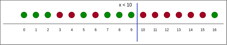 The entropy of these two groups:
\[
\begin{equation}
S_l = - \frac{3}{10}log_2\frac{3}{10} - \frac{7}{10}log_2\frac{7}{10} = 0.8812908992306927
\end{equation}
\]
\[
\begin{equation}
S_r = - \frac{6}{7}log_2\frac{6}{7} - \frac{1}{7}log_2\frac{1}{7} = 0.5916727785823275
\end{equation}
\]
The entropy value has decreased in both groups. It means our strategy of splitting results in
two more ordered groups.
Information gain:
\[
\begin{equation}
IG = S_0- \frac{10}{17}S_l - \frac{7}{17}S_r = 0.23546616740539644.
\end{equation}
\]
We can continue to split the dataset into groups in the way in which we are until
the circles in each group are all of the same color.
The entropy of these two groups:
\[
\begin{equation}
S_l = - \frac{3}{10}log_2\frac{3}{10} - \frac{7}{10}log_2\frac{7}{10} = 0.8812908992306927
\end{equation}
\]
\[
\begin{equation}
S_r = - \frac{6}{7}log_2\frac{6}{7} - \frac{1}{7}log_2\frac{1}{7} = 0.5916727785823275
\end{equation}
\]
The entropy value has decreased in both groups. It means our strategy of splitting results in
two more ordered groups.
Information gain:
\[
\begin{equation}
IG = S_0- \frac{10}{17}S_l - \frac{7}{17}S_r = 0.23546616740539644.
\end{equation}
\]
We can continue to split the dataset into groups in the way in which we are until
the circles in each group are all of the same color.
Usually we deal with multicategorial data represented as table(s). In each step ID3 algorithm choses the attribute with the largest information gain as the decision node.
1.2 Gini index (or Gini impurity)
Another splitting criteria is based on Gini Index. It is used in the CART algorithm. Gini index is a measure of particular element being wrongly classified when it is randomly chosen. Let’s say $p_i$ is the probability of object being classified to a particular class, then \[ \begin{equation} G = \sum^{C}_{i=1} p_i \large ( \sum_{k \neq i}^{C} p_k\large ) = \sum^{C}_{i=1} p_i(1 - p_i), \end{equation} \]
\[ \begin{equation} G = 1 - \sum^{C}_{i=1}p_i^2 \end{equation} \]
It is easy to see that $G=0$ if all observations belong to the same class (label). Gini Index and Entropy can be used interchangeably.
Gini based splitting favors larger partitions. Entropy that have small counts but many distinct values.
1.3 How to work with different types of features
Common notes:
- if chosen splitting feature does not give us a reduction in impurity score, we do not use this feature
- to handle with overfitting we could have used a threshold such that impurity reduction has to be large enough
Numeric feature type:
- sort elements by feature value
- calculate the average feature value for all adjacent elements
- calculate splitting criteria value for each average feature values
- choose the best splitting criteria value
Categorical data, ranked data:
- calculate splitting criteria for each feature value
- choose the best splitting criteria value
2. Regression tree.
Let us consider, as an example how the amount of fertilizers influence growth rate of vegetables.
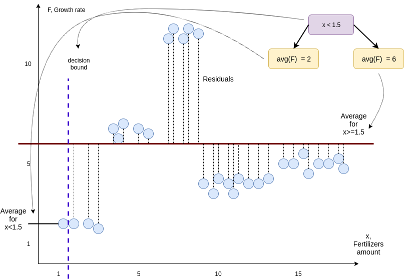
Consider very simple decision tree that splits our measurements into two groups based on whether or not $x < 1.5$. The average growth rate on the left is $2$. The average growth rate on the right side is $6$. These two values are the predictions that our decision tree will make.
To quantify the quality of these predictions we will calculate the sum of squared residuals (differences between the observed and the predicted values).
On the next picture we can see that our new decision bound results in a smaller sum of squared residuals.
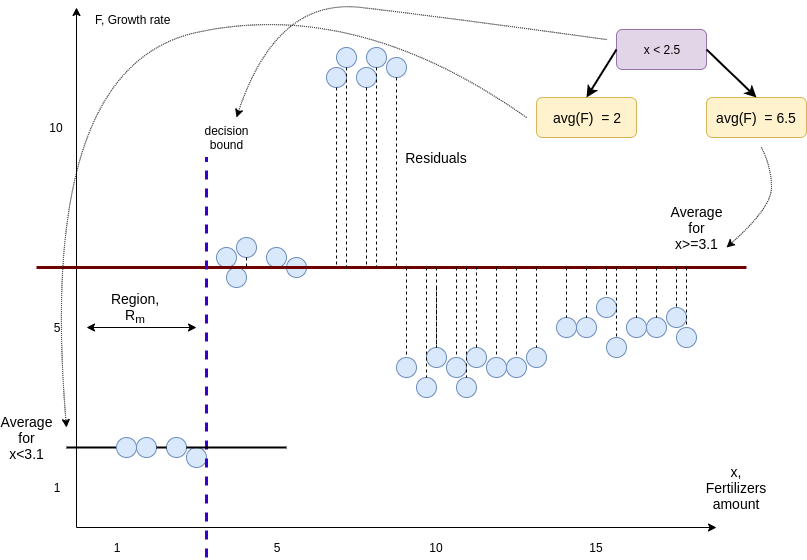
We continue moving our decision boundary until we have calculated the sum of squared residuals for all remaining thresholds. And then threshold resulting in smallest sum of squared residuals is used as the root of our tree: \[ \begin{equation} \sum (y_i - F(x_i))^2 \rightarrow min \end{equation} \]
Model’s prediction is:
\[ \begin{equation} F(x) = \sum_{m-1}^{M}c_m I(x \in R_m) \end{equation} \]
where $c_m$ is the response in $m$-th region. $I$ indicates that $x$ belongs to the region $R_m$.
To build regression tree we recursively apply the same procedure for observations that ended up in the node to the left and right of the root.
2.1 How to prevent overfitting. Regression trees pruning.
- do splitting only if number of observations more than some minimum number
- pruning
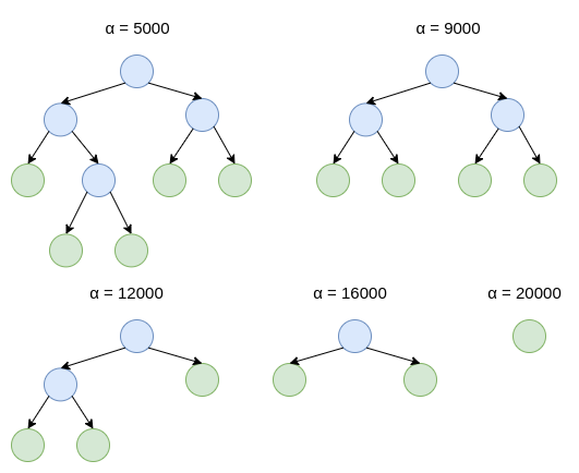
Cost complexity pruning
We can prune a tree by removing some of the leaves and replacing the parent node with a leaf that is the average of removed nodes. We define cost complexity criteria or tree score:
\[ \begin{equation} C(T) = SSR + \alpha |T| \end{equation} \] where $SSR$ is the sum of squared residuals, $\alpha >= 0$ - tunning parameter (we find it using cross-validation). $|T|$ - the number of terminal nodes or leaves in tree $T$.
The idea is to find, for each $\alpha$ a subtree to minimize $C(T)$.
To do that do the following steps:
-
build the full sized regression tree by fitting it on all of the data (not just the training data). (increase $\alpha$ until pruning leaves will give us a lower tree score and use the resulting subtree) $\times N$. In the end different values of $\alpha$ give us a sequence of trees, from full sized to just a leaf
- split data into training and validation data sets. Just using the training data use the $\alpha$ values we found before to build a full tree and a sequence of sub-trees that minimize the tree score. Use the validation data to calculate the $SSR$s for each new tree. 10-fold cross-validation. The final value of $\alpha$, on average, gives us the lowest $SSR$ with the validation data.
- go back to the trees from 1 and pick the tree that corresponds to the final value from 2