Support Vector Machines
Linear SVM
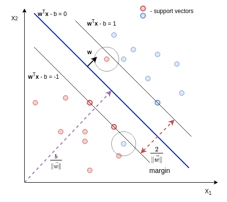
Support Vector Machine performs classification by finding the optimal separating hyperplane that maximizes the margin between the two classes (OSH is as far as possible from the data points of each category).
We are given a set of data points $\{(\mathbf{x}_1, y_1), \dots (\mathbf{x}_n, y_n)\}$, where $y_i \in \{-1, 1\}$ and $\mathbf{x}_i$ are vectors (usually normalized). We are looking for hypothesis $h(\mathbf{x}) = sign(\mathbf{w}^T\mathbf{x}-b)$.
A hyperplane can be defined by \[ \begin{equation} \mathbf{w}^T\mathbf{x} - b = 0 \tag{0}\label{0} \end{equation} \]
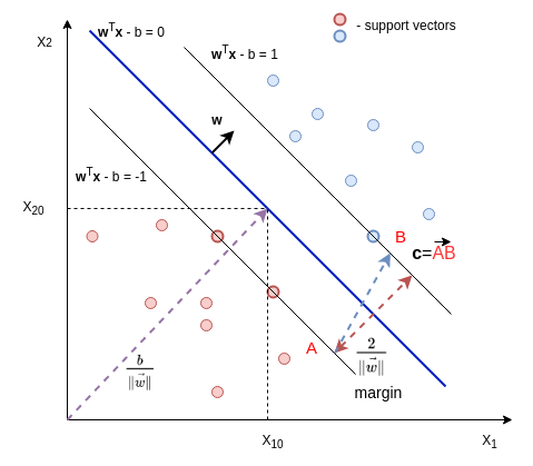
where $\mathbf{w}$ is the normal vector to the hyperplane. $\frac{b}{\Arrowvert \mathbf{w} \Arrowvert}$ is the distance from the origin to the hyperplane (proof: $\mathbf{z} = (x_{10}, x_{20})$, $d = proj_{\mathbf{w}}\mathbf{z} = \frac{\mathbf{w} \cdot \mathbf{z}}{\Arrowvert \mathbf{w} \Arrowvert} = \frac{b}{\Arrowvert \mathbf{w} \Arrowvert}$).
Linearly separable data (hard-margin)
To find optimal separating hyperplane we can select two parallel hyperplanes that separate two categories,
so that the distance between them as large as possible
\[
\begin{split}
\mathbf{w}^T \mathbf{x} - b &= 1 \\
\mathbf{w}^T \mathbf{x} - b &= -1
\end{split} \tag{1}\label{eq1}
\]
The distance between these two hyperplanes is $\frac{2}{\Arrowvert \mathbf{w} \Arrowvert}$.
(proof: $d = proj_{\mathbf{w}}\mathbf{c} = \frac{\mathbf{w} \cdot \mathbf{c}}{\Arrowvert \mathbf{w} \Arrowvert} = \frac{(\mathbf{B} - \mathbf{A})\cdot \mathbf{w}}{\Arrowvert \mathbf{w} \Arrowvert} = \frac{(\mathbf{B}\mathbf{w} - \mathbf{A}\mathbf{w})}{\Arrowvert \mathbf{w} \Arrowvert} = \frac{b+1 -b+1}{\Arrowvert \mathbf{w} \Arrowvert} = \frac{2}{\Arrowvert \mathbf{w} \Arrowvert}$)
The margin is given by $M = y(\mathbf{w}^T \mathbf{x}-b)$. $M$ is negative only if the model misclassifies an object.
Now we can define an optimization problem to find optimal margin classifier:
\[
\begin{split}
&\frac{1}{2}{\Arrowvert \mathbf{w} \Arrowvert}^ 2 \rightarrow \min \\
&subject\;to\; y_i(\mathbf{w}^T \mathbf{x}-b) \geqslant 1, \;i=1\dots m
\end{split} \tag{2}\label{eq2}
\]
To solve this optimization problem we recast it in dual form. The Lagrangian function is defined as \[ \begin{equation} L(\mathbf{w},b,\alpha)=\frac{1}{2}\Arrowvert \mathbf{w} \Arrowvert^2-\sum_{i=1}^{m}{\alpha_i[y_i(\mathbf{w}\cdot \mathbf{x_i} - b)-1]} \tag{3}\label{eq3} \end{equation} \] and the Lagrangian primal problem
\[
\begin{split}
&\min_{\mathbf{w},b}\space \max L(\mathbf{w},b,\alpha) \\
&subject \space to \space \alpha_i \ge 0, i=1\dots m
\end{split} \tag{4}\label{eq4}
\]
Calculating the derivatives of Lagrangian and assuming them to be a zero we get:
\[
\begin{split}
&\nabla_w L(\mathbf{w},b,\alpha) = \mathbf{w} - \sum_{i=1}^{m}{\alpha_iy_i \mathbf{x_i}}=0 \\
&\nabla_b L(\mathbf{w},b,\alpha) = -\sum_{i=1}^{m}{\alpha_iy_i}=0
\end{split} \tag{5}\label{eq5}
\]
From the above two equations, we get $\mathbf{w}=\sum_{i=1}^{m}{\alpha_iy_i\mathbf{x_i}}$. Substituting it to $(\ref{eq3})$ we get \[ \begin{equation} W(\alpha)= \sum_{i=1}^m\alpha_i -\frac{1}{2}\sum_{i=1}^m\sum_{j=1}^m\alpha_i\alpha_jy_iy_j(\mathbf{x_i}\cdot \mathbf{x_j}) \tag{6}\label{6} \end{equation} \]
The dual problem is thus stated as:
\[
\begin{split}
&\max_\alpha \sum_{i=1}^m\alpha_i -\frac{1}{2}\sum_{i=1}^m\sum_{j=1}^m\alpha_i\alpha_jy_iy_j(\mathbf{x_i}\cdot \mathbf{x_j}) \\
& subject\space to\space \alpha_i \ge 0, i=1\dots m, \sum_{i=1}^m{a_iy_i}=0
\end{split} \tag{7}\label{eq7}
\]
Solving the last problem we get $\alpha_i$. Now we can calculate $\mathbf{w}=\sum_{i=1}^{m}{\alpha_iy_i\mathbf{x_i}}$ and $b = \frac{1}{S}\sum_{i=1}^S(y_i-\mathbf{w}\cdot \mathbf{x_i})$, where $S$ is the number of support vectors.
The problem with hard-margin SVM is that it does not work with linearly inseparable data.
Linearly inseparable data (soft-margin)
Nonlinear classification. Kernel trick
Noisy data
To tackle the problem with linearly inseparable data caused by outliers (noisy data) we modify our equations ($\ref{eq2}$) introducing slack variables $\psi_i$:
\[
\begin{split}
&\min_{w,b,\psi}\frac{1}{2}\Arrowvert \mathbf{w} \Arrowvert + C\sum_{i=1}^{m}\psi_i\\
&subject\;to\; y_i(\mathbf{w}^T \mathbf{x}-b) \geqslant 1 - \psi_i, \; \psi_i \ge 0 \;i=1\dots m
\end{split} \tag{8}\label{eq8}
\]
We add $\psi_i \ge 0$ to prevent the optimization by using negative values.
$C$ is regularization parameter. It controls how mach we want to avoid misclassifications. Increasing $C$ contributes to smaller margin.
Dual problem is defined as
\[
\begin{split}
&\max_\alpha \sum_{i=1}^m\alpha_i -\frac{1}{2}\sum_{i=1}^m\sum_{j=1}^m\alpha_i\alpha_jy_iy_j(\mathbf{x_i}\cdot \mathbf{x_j}) \\
&subject\space to\space 0 \le \alpha_i \le C, i=1…m, \sum_{i=1}^m{a_iy_i}=0
\end{split} \tag{9}\label{eq9}
\]
Kernel Trick
There are situations where a nonlinear region can separate the groups more efficiently.
The idea is to use replace the dot-product $(\mathbf{x_i}\cdot \mathbf{x_j})$ with
a kernel function $K(x_i,x_j)$
\[
\begin{split}
&\max_\alpha \sum_{i=1}^m\alpha_i -\frac{1}{2}\sum_{i=1}^m\sum_{j=1}^m\alpha_i\alpha_jy_iy_j K(x_i,x_j) \\
&subject\space to\space 0 \le \alpha_i \le C, i=1…m, \sum_{i=1}^m{a_iy_i}=0
\end{split} \tag{10}\label{eq10}
\]
We can think of it like dot product is performed in another space. We now have the ability to change the kernel function in order to classify non-linearly separable data.