Backpropagation in neural networks. Activation functions.
Math behind backpropagation
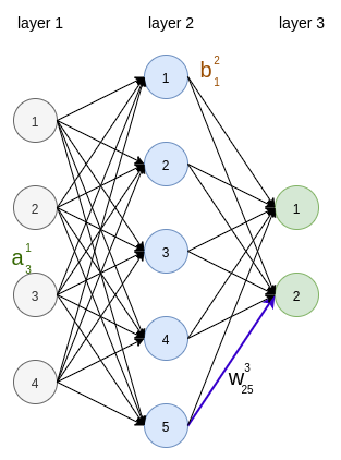
Let us start with a notation which we will use in the explanation.
- $w_{jk}^l$ is the weight of connection from node $k$ in the layer $l - 1$ to node $j$ in the next layer
- $b_j^l$ is the bias for node $j$ in the layer $l$
- $a_j^l$ is the activation of $j$-th neuron in the layer $l$
- E is the cost function
The goal of backpropagation is to minimize the cost function $E$ by computing the partial derivatives $\frac{\partial E}{\partial w}$ and $\frac{\partial E}{\partial b}$ with respect to any weight and bias in the network.
The activation of a neuron in the $l$-th layer depends on activations of neurons in the layer $l-1$ \[ \begin{equation} a_j^l = \sigma(\sum_{k \in layer_{l-1} } w_{jk}^l a_k^{l-1} + b_j^l), \end{equation} \] or \[ \begin{equation} a_j^l = \sigma(z_j^l), \; z_j^l = \sum_{k \in layer_{l-1} } w_{jk}^l a_k^{l-1} + b_j^l \tag{1}\label{eq1} \end{equation} \]
We define a error of $j$-th neuron on the $l$-th layer:
\[ \begin{equation} \delta^l_j = \frac{\partial E}{\partial z^l_j} \tag{2}\label{eq2} \end{equation} \]
An equation for the error in the output layer
\[ \begin{equation} \boxed{\delta^L_j = \frac{\partial E}{\partial z^L_j} = \frac{\partial E}{\partial a^L_j} \frac{\partial a^L_j}{\partial z^L_j} = \frac{\partial E}{\partial a^L_j} \sigma’(z_j^L)} \tag{3}\label{eq3} \end{equation} \]
Now we reformulate the expression $(\ref{eq2})$ for $\delta^l_j$ in terms of the error in the next layer $l+1$:
\[
\begin{split}
\delta^l_j &= & \frac{\partial E}{\partial z^l_j} \\
&= & \sum_k \frac{\partial E}{\partial z^{l+1}_k} \frac{\partial z^{l+1}_k}{\partial z^l_j} \\
&= & \sum_k \frac{\partial z^{l+1}_k}{\partial z^l_j} \delta^{l+1}_k
\end{split} \tag{4}\label{eq4}
\]
Note that: \[ \begin{equation} z_k^{l+1} = \sum_{j} w_{kj}^{l+1} \sigma(z_j^l) + b_k^{l+1} \tag{5}\label{eq5} \end{equation} \]
Putting $(\ref{eq5})$ to $(\ref{eq4})$ we get :
\[ \begin{equation} \boxed{\delta^l_j = \sum_{k} \delta_k^{l+1} w_{kj}^{l+1} \sigma’(z_j^l)} \tag{6}\label{eq6} \end{equation} \]
Rate of change of the cost function with respect to a weight in network: \[ \begin{equation} \boxed{\frac{\partial E}{\partial w_{jk}^l} = \frac{\partial E}{\partial z_j^l} \frac{\partial z_j^l}{\partial w_{jk}^l} = \delta_j^l a_k^{l-1}}\tag{7}\label{eq7} \end{equation} \]
Rate of change of the cost function with respect to a bias in network: \[ \begin{equation} \boxed{\frac{\partial E}{\partial b_j^l} = \frac{\partial E}{\partial z_j^l} \frac{\partial z_j^l}{\partial b_j^l} = \delta_j^l }\tag{8}\label{eq8} \end{equation} \]
Equations $(\ref{eq3})$, $(\ref{eq6})$, $(\ref{eq7})$, $(\ref{eq8})$ are fundamental equations of backpropagation.
Backpropagation algorithm
Let’s say we have some network with $n$ layers.
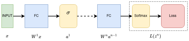
For each layer we calculate $a^l$ and $z^l$. Doing backpropagation our goal is to calculate the derivatives of loss function with respect to parameters $w^l$ going from the end of network back to the front.
- So we start at the end and calculate $\delta = \frac{dL}{dz^n}$.
- Then for each function $f$ in network with input $x_f$ and parameters $\theta_f$ from start to end:
\[ \begin{equation} \frac{dL}{d\theta_f} = \frac{df}{d\theta_f}\delta \end{equation} \]
- then we update $\delta$: \[ \begin{equation} \delta \leftarrow \frac{df}{dx_f}\delta \end{equation} \]
Here is an example for shallow 2-layer network.
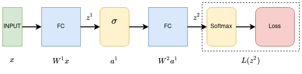
\[ \begin{equation} \frac{dL}{dW^2} = \frac{dz^2}{dW^2}\frac{dL}{dz^2} \end{equation} \]
\[ \begin{equation} \frac{dL}{dW^1} = \frac{dz^1}{dW^1}\frac{da^1}{dz^1}\frac{dz^2}{da^1}\frac{dL}{dz^2} \end{equation} \]
Vanishing gradients problem
As more layers are added to a network, the gradients of a loss function approaches zero. In practice we can observe that layers closest to the output of the network learn faster then deeper layers.
On the picture below is an example of simple 4-neuron network.
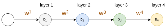
Let us calculate the gradient $\frac{\partial E}{\partial w^1}$:
\[ \begin{equation} \frac{\partial E}{\partial w^1} = \frac{\partial E}{\partial a^4} \frac{\partial a^4}{\partial z^4} \frac{\partial z^4}{\partial a^3} \frac{\partial a^3}{\partial z^3} \frac{\partial z^3}{\partial a^2} \frac{\partial a^2}{\partial z^2} \frac{\partial z^2}{\partial a^1} \frac{\partial a^1}{\partial z^1}, \end{equation} \]
\[ \begin{equation} \frac{\partial E}{\partial w^1} = \frac{\partial E}{\partial a^4} \sigma’(z^4) w^4 \sigma’(z^3) w^3 \sigma’(z^2) w^2 \sigma’(z^1) \end{equation} \]
The maximum of the derivative of the sigmoid function is $0.25$. If the weights $w^i$ are less than $1$ the right side of equation will exponentially decrease.
Activations
- Sigmoid $\sigma(x) = \frac{1}{1 + \exp(x)}$
- saturated neurons zeros out the gradients
- non zero centered
- $exp$ is computationally expensive
- $tanh(x) = \frac{\exp(x) - \exp(-x)}{\exp(x) + \exp(-x)}$
- saturated neurons zeros out the gradients
- squashes input to range $[-1, 1]$
- zero centered
- $ReLU(x) = max(0, x)$
- non-zero derivative if $x > 0$
- computationally cheap
- not zero centered
- $Leaky\;ReLU(x) = max(0.01x, x)$
- non-zero derivative
- $Exponential\;ReLU(x) = x \; if \; x > 0 \;else \; \alpha(exp(x) - 1)$
- non-zero derivative